Lab 8: Spectral Signature Analysis & Resource Monitoring

Goals and Background: 

The main goal of this lab is for you to gain experience on the measurement and interpretation of spectral reflectance (signatures) of various Earth surface and near surface materials captured by satellite images and also to perform basic monitoring of Earth resources using remote sensing band ratio techniques. In this lab, you will learn how to collect spectral signatures from remotely sensed images, graph them, and perform analysis on them to verify whether they pass the spectral separability test discussed in lectures. This is a prerequisite for image classification which will be cover in the advanced version of this class. Also you will monitor the health of vegetation and soils using simple band ratio techniques. At the end of this lab, students will be able to collect and properly analyze spectral signature curves for various Earth surface and near surface features for any multispectral remotely sensed image and also monitor the health of vegetation and soils.

Methods:

Spectral signature analysis

A spectral signature is a graphical representation of the spectral response of a certain type of feature or object as a function of wavelength. Basically, a spectral signature indicates which bands are reflected the most in a surface feature.

The spectral signatures analyzed in this lab are as follows:


1. Standing Water
2. Moving water
3. Vegetation
4. Riparian vegetation.
5. Crops
6. Urban Grass
7. Dry soil (uncultivated)
8. Moist soil (uncultivated)
9. Rock
10. Asphalt highway
11. Airport runway
12. Concrete surface (Parking lot)

In order to capture the spectral signatures, the surface feature was found on the imagery and a polygon (found under the drawing toolbar) was created (figure 1).

Figure 1. Capturing Lake Wissota's spectral signature by creating a polygon on the surface feature.

The spectral signature window was accessed through the Raster tab and then Supervised  and Signature Editor. After the window was opened, the new signature was added to the table (figure 2). Sometimes, it was difficult to discern the individual features on the false color imagery, so Google Earth was linked to ERDAS, which made determining features much easier.

Figure 2. All 12 of spectral signatures added in the Signature Editor table. Statistics could also be viewed from this window.

Spectral signatures are useful in being able to detect differences between surface features, such as dry and moist soil. Although they are very similar surface features, their moisture content determines reflectivity, and ultimately the spectral signature of the soils (figure 3).

Figure 3. Spectral signatures of dry soil and moist soil. Moisture content is one of the main determinants of spectral signature in soil. The higher the moisture content, the lower the reflectance. This is 'reflected' in the spectral signature of water, which has low reflectance comparatively to other signatures. 

Resource monitoring

Resource monitoring is an extremely practical use of remote sensing, and is of great interest to many people, including farmers and urban planners. Using remote sensing for these types of applications is much less expensive and convenient than individually examining plants or soil for health of resources. In this lab we will examine two of the many calculations that can easily be done in ERDAS: NDVI and FM.

Normalized difference vegetation index (NDVI) is used to determine vegetation abundance in imagery. The equation for this calculation is NDVI = (NIR-Red)/(NIR + Red) where NIR is near infrared and Red is the red band (band 3). In ERDAS, this calculation can be done simply by accessing the Raster tab, then Unsupervised, then NDVI.

Detecting ferrous minerals (FM) is important in examining the health of soil, and for agricultural regions, crop fields. The equation for calculating FM = MIR/NIR, where MIR is middle infrared and NIR is near infrared. In ERDAS, this calculation can be done simply by accessing the Raster tab, then Unsupervised, then Indices, then select the ferrous mineral option from the index dropdown.

Results:

The running list of all 12 spectral signatures created above were added to the Spectral Signature window, and a graph could be created to analyze the differences between the feature's signatures. Below depicts the spectral signatures and how they coincide with one another (figure 4).

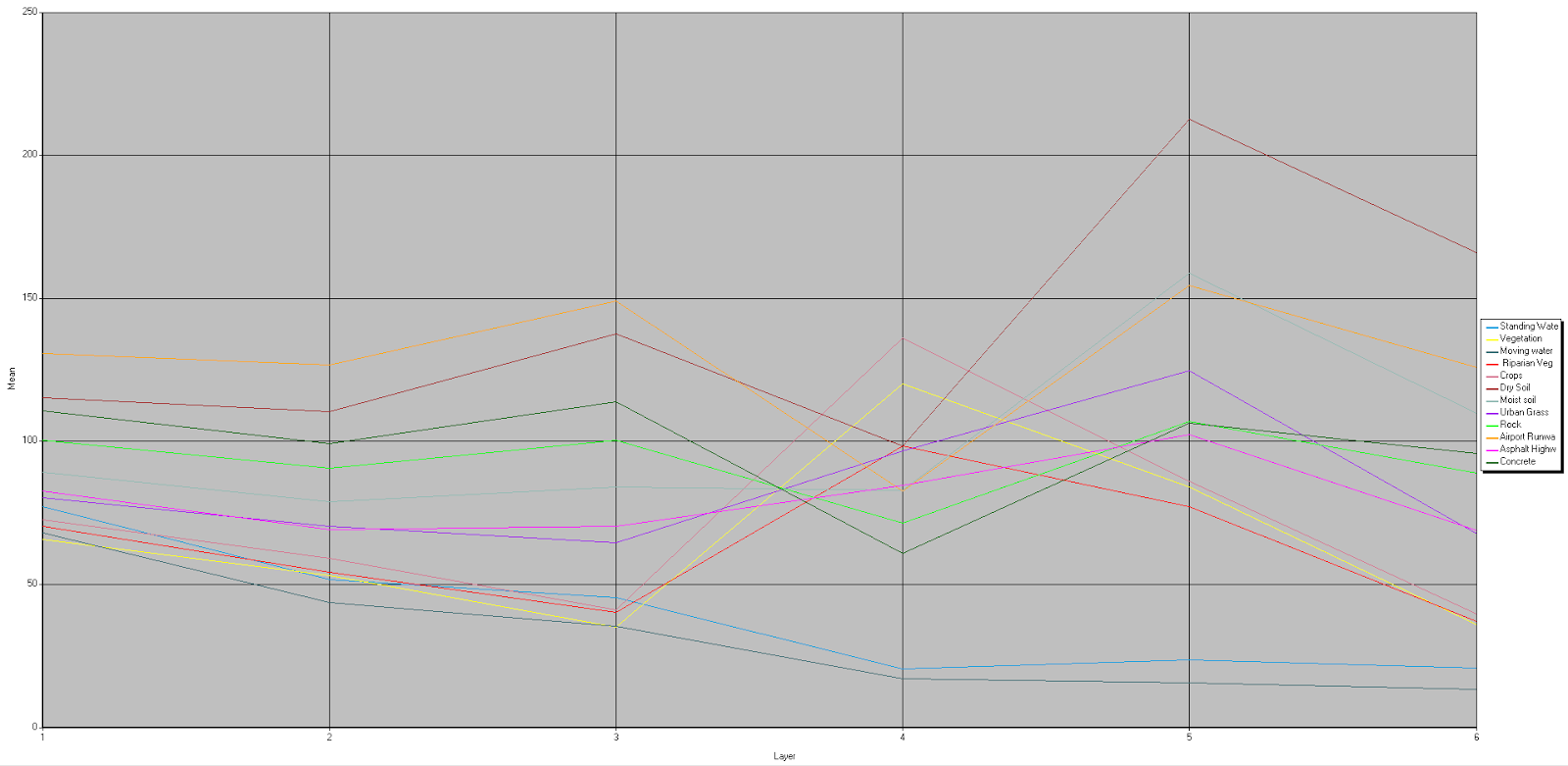Figure 4. Spectral signatures. The y-axis highlights the percentage of reflectance and the x-axis depicts the bands at each tick mark (e.g Band 1 = 1 etc).

After using the NDVI calculator, the displayed image in ERDAS was black and white, not so exciting or helpful, so ArcMap was used to classify discrete values and create an informative map of Eau Claire and Chippewa counties (figure 5).

Figure 5. NDVI map of Eau Claire and Chippewa Counties in 2000.

Similar to the NDVI, the FM calculator was utilized and the imagery was brought into ArcMap to be displayed in a cartographically pleasing manner. Maps like this can be very useful for farmers who are curious of the iron content of their soil (figure 6).

Figure 6. Ferrous Mineral Content of Eau Claire and Chippewa Counties in 2000.

Conclusion:

I really loved doing this lab. We have been talking about reflectance throughout the semester, and creating our own spectral signatures was in a very nerdy way, quite rewarding. Understanding spectral signatures is vital in being able to effectively identify vegetation types. Doing this lab has also given me a new appreciation for landcover identification. I also really enjoyed calculating NDVI and ferrous minerals. Although this lab is relatively simple compared to orthorectification, learning these tools will help immensely in the future.

Source:

Satellite image is from Earth Resources Observation and Science Center, United States Geological Survey.