Lab 4: Miscellaneous Image Functions

Goals and Background:

There are seven main learning objectives in this lab which include:

1) delineating a study area from a larger satellite image scene
2) demonstrating how spatial resolution of images can be optimized for visual interpretation purposes
3) introducing some radiometric enhancement techniques in optical images
4) linking a satellite image to Google Earth which can be a source of ancillary information
5) introducing students to various methods of resampling satellite images
6) exploring image mosaicking
7) exposing students to binary chance detection with the use of simple graphical modeling

These objectives will aid in the understanding of basic remote sensing concepts, which will provide a gateway to more advanced techniques for future projects.

Methods:

Subsetting an image with an Inquire Box and area of interest (AOI) shapefile.

Most often, the extent of a .img file is not sufficient for the desired study area. Reducing the extent of the image allows for quicker analysis and processing of the imagery. The Inquire Box allows the user to limit the extent of the study area by simply drawing a box around the approximate area (figure 1), the output image is found in figure 7.

Figure 1. Subsetting with the use of an Inquire Box. Note the box located in the upper right corner of the image in red; this is the extent of the Inquire Box for this section. 

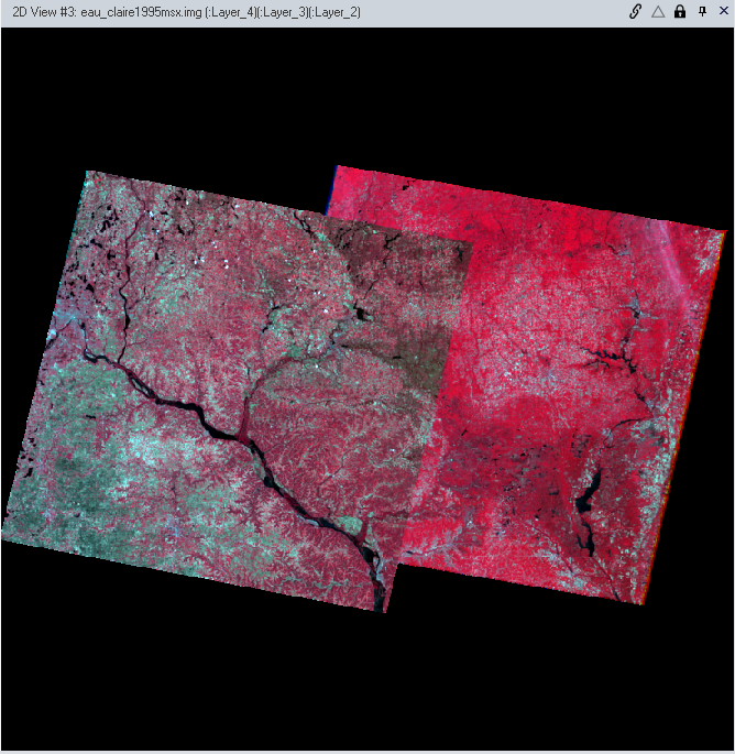
Often times, drawing an Inquire Box is not precise enough for an analysis-after all, how often do you have a perfect rectangle as an AOI? This is when subsetting using an AOI shapefile comes into play. The shapefile is brought into ERDAS Imagine and saved as an AOI file (figure 2). The tool 'Subset and Chip', found under the Raster toolbar will remove the rest of the image and leave only the desired area of the shapefile (output image is found in figure 8).

Figure 2. Eau Claire and Chippewa counties shapefile on top of the .img file. 

Part 2: Image Fusion

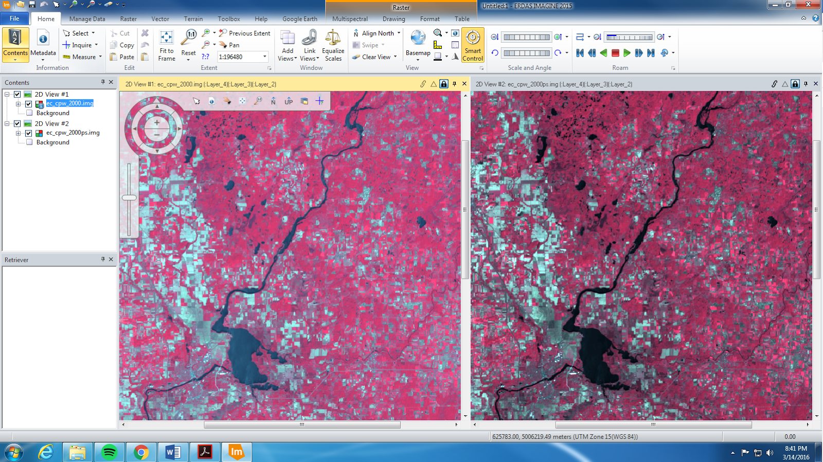
Pansharpening is a tool that optimizes the image for spatial resolution by combining the panchromatic band with a higher spatial resolution with lower resolution multispectral imagery. For the data in this lab, the multispectral image had a resolution of 30 meters and the panchromatic image had a resolution of 15 meters.

In order to use this method, one must resample the data to merge the resolution. This is found under the Pan Sharpen tab (output images are found in figures 9 and 10).

Part 3: Simple Radiometric Enhancement Techniques

Various steps can be taken to improve image and radiometric quality. One such improvement is reducing haze in imagery. This can be done by accessing the Raster tab and within it the Radiometric button, followed by the drop down menu's Haze Reduction button. The haze reduction enhancement increases the brightness values, thus allowing a better analysis to occur on the imagery (output images are found in figures 11 and 12).

Part 4: Linking Image Viewer to Google Earth

Sometimes it can be difficult to discern what certain shapes are in an .img file. Google Earth can often solve that mystery by providing labels for many of their landmarks. This application is accessed via the Google Earth tab, followed by the Connect to Google Earth button, then Match GE to View and Sync GE to View. This allows the user to easily determine what it is they're actually seeing in ERDAS because Google Earth displays labels, photos, and other indicators for determining individual areas in an image (figure 3).

Figure 3. Linked ERDAS and Google Earth Imagery. Without Google Earth, it would be much more difficult to 

Part 5: Resampling

In order to analyze imagery properly, it is important to have the same pixel size. Changing pixel size is completed by the process of resampling. Resampling can be done 'up' or 'down' depending on the type of analysis required. Resampling can be done by selecting the Raster tab, followed by the Spatial button and then the drop down menu will contain the Resample Pixel Size button. Two of the four types of resampling methods were performed: Nearest Neighbor (output image in figure 13) and Bilinear Interpolation (output image in figure 14). Both methods were resampled from 30 x 30 meters to 15 x 15 meters.

Part 6: Image Mosaicking

Once determining a study area, there is a good chance that the study area is located in multiple .img files. This requires the user to mosaic two or more images into one 'seamless' layer. This can be done using a couple of different methods: Mosaic Express and Mosaic Pro. Mosaic Express provides a simple visual display, but no analysis should be conducted from this imagery.The Mosaic Express does not chance the brightness settings, but rather simply matches up the latitude/longitude to line up and overlap the images (output image in figure 15).

Mosaic Pro takes into account multiple facets including Histogram Matching, setting output options, and setting overlap functions, just to name a couple factors. The output of the Mosaic Pro image shows basically homogenous brightness and provides enough information in its imagery to be more useful for analysis (output image in figure 16).

Part 7: Binary Change Detection (image differencing)

So far in the course, no actual analysis has taken place, largely because we've needed the tools to get to the point in which analysis can take place. Binary change detection is the first small victory in analysis in remote sensing. This process takes the brightness values from two different images from Eau Claire County, in this case one from 1991 and one from 2011, and compares how they have changed over time. In order to do the analysis, I needed to click on the Raster tab --> Scientific --> Functions --> Two Image Functions --> Two Image Operators. The areas of change normally happen at the very tails of histograms, so the rule of thumb threshold of mean + 1.5 standard deviation will be used, the estimated threshold is depicted below (figure 4). In order to detect the change, a new histogram must be established that changes the values from + to only -.

Figure 4. Rule of thumb threshold values calculated by using the mean + 1.5 standard deviation of the mean. The upper limit of the change/no change threshold is highlighted (yy) as well as the lower limit of the change/no change threshold (-xx)

A model was run to eliminate the negative values in the difference image created previously. The model was provided to the class by Dr. Cyril Wilson (figure 5).

Figure 5. Model to eliminate the negative values in the difference image created previously.  

Model Maker was used to perform the binary change detection. The inputs for the model were the 1991 and 2011 images. The function was the 2011 input - 1991 input + 127 (which was the constant) (figure 6).

Figure 6. Model Maker for binary change detection in Eau Claire County.

The output image resulted in a map depicting only the changed pixels (output image in figure 17). The only issue with this analysis is that one cannot know if the change was 'positive' or 'negative', but simply that it does not have the same value it held previously.

Results:

The results of my methods are displayed below:

Image Subset: 

Figure 7. The subset produced via the Inquire Box

Figure 8. The subset AOI after using the 'Subset and Chip' tool. Note Eau Claire and Chippewa counties are combined.

Image Fusion (Pansharpen):

Figure 9. Pansharpened vs. non-pansharpened image comparison. The non-pansharpened image is on the left viewer, and the pansharpened image is on the right viewer. Note the difference in brightness values. The pansharpened image depicts a greater contrast in brightness.

Figure 10. Zoomed-in version of pansharpened vs non-pansharpened images.

Haze Reduction:

Figure 11. Pre-haze reduction (left) and post-haze reduction (right). Notice the brightness values in the haze reduced image.

Figure 12. Zoomed-in version of non-haze reduced (left) and haze reduced (right) images.

Image Resampling:

Figure 13. Comparative of regular image on left and Nearest Neighbor resampling on the right. Note the 'stair step' pattern that the Nearest Neighbor resampling creates.

Figure 14. Comparative of regular image on left and Bilinear Interpolation on the right. 

Image Mosaicking: 

Figure 15. Mosaicing using the Mosaic Express method. Note the colors for the two original .img files are not cohesive after this method. This method is only to be used to obtain surface level information and no analysis should be conducted with this method.

Figure 16. Mosaicing using the Mosaic Pro method. Note the colors of the two original images is basically seamless now.

Binary Change Detection:

Figure 17. The final output map for Binary Change detection from 1991 and 2011 in Eau Claire County.

Conclusion:

In order to be able to analyze ERDAS imagery, numerous tools are required to make the imagery usable. A few of the tools were explored in this lab. Not only do they make the imagery usable, but they allow for a better analysis. In addition, the first elementary analysis using binary change detection was completed. This provides a gateway for future remote sensing analysis.

Sources:

• Satellite images are from Earth Resources Observation and Science Center, United States Geological Survey (USGS)
• Shapefile is from Mastering ArcGIS 6th Edition Dataset by Maribeth Price, McGraw Hill. 2014.